Q-learning on a three columns dataset
Overview
In this example, we use a tabular Q-learning algorithm to anonymize a data set with three columns. In particular, we discretize the total dataset distortion into bins. Another approach could be to discretize the distortion of each column into bins and create tuples of indeces representing a state. We follow the latter approach in another example.
Q-learning
Q-learning is one of the early breakthroughs in the field of reinforcement learning [1]. It was first introduced in [2]. Q-learning is an off-policy algorithm where the learned state-action value function \(Q(s, \alpha)\) directly approximates the optimal state-action value function \(Q^*\). This is done independently of the policy \(\pi\) being followed [1].
The Q-learning algorithm is an iterative algorithm where we iterate over a number of episodes. At each episode the algorithm steps over the environment for a user-specified number steps it executes an action which results in a new state. This is shown collectively in the image below
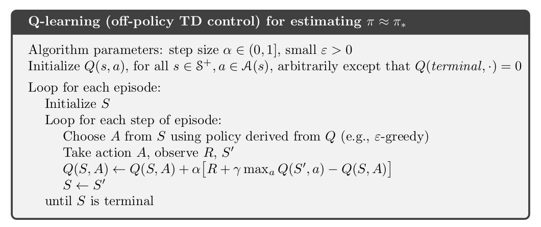
Q-learning algorithm. Image from [1].
At each episode step, the algorithm updates \(Q(s, \alpha)\) according to:
where \(\alpha\) is a user-defined learning factor and \(\gamma\) is the user-defined discount factor. The algorithm requires the following user-defined input
Number of episodes
Number of steps per episode
\(\gamma\)
\(\alpha\)
An external policy function to decide which action to take (e.g. \(\epsilon\)-greedy)
Although with Q-learning \(Q(s, \alpha)\) directly approximates \(Q^*\) independently of the policy \(\pi\) being followed, the policy still has an effect in that it determines which state-action pairs and visited updated. However, for correct convergence all that is required is that all pairs continue to be updated [1]. In fact, any method guaranteed to find optimal behavior in the general case must require it [1].
The algorithm above, stores the expected value estimate for each state-action pair in a table. This means we cannot use it when we have continuous states or actions, which would lead to an array of infinite length. Given that the total dataset distortion is assumed to be in the range \([0, 1]\) of the real numbers; where the edge points mean no distortion and full distortion of the data set/column respectively. We discretize this range into bins and for each entailed value of the distortion we use the corresponding bin as a state index. Alternatively, we could discretize the distortion of each column into bins and create tuples of indeces representing a state.
We preprocess the data set by normalizing the numeric columns. We will use the cosine normalized distance to measure the distortion of columns with string data. Similarly, we use the following \(L_2\)-based norm for calculating the distortion of numeric columns
where $N$ is the size of the vector. This way the resulting distance, due to the normalization of numeric columns, will be in the range \([0,1]\).
Code
The necessary imports
import numpy as np
import random


from src.trainers.trainer import Trainer, TrainerConfig
from src.algorithms.q_learning import QLearning, QLearnConfig
from src.spaces.action_space import ActionSpace
from src.spaces.actions import ActionIdentity, ActionStringGeneralize, ActionNumericBinGeneralize
from src.policies.epsilon_greedy_policy import EpsilonGreedyPolicy, EpsilonDecayOption
from src.utils.iteration_control import IterationControl
from src.examples.helpers.plot_utils import plot_running_avg
from src.datasets import ColumnType
from src.examples.helpers.load_three_columns_mock_dataset import load_discrete_env, \
    get_ethinicity_hierarchy, get_salary_bins, load_mock_subjects
from src.spaces.env_type import DiscreteEnvType
from src.utils import INFO
Next establish a set of configuration parameters
# configuration params
EPS = 1.0
EPSILON_DECAY_OPTION = EpsilonDecayOption.CONSTANT_RATE  # .INVERSE_STEP
EPSILON_DECAY_FACTOR = 0.01
GAMMA = 0.99
ALPHA = 0.1
N_EPISODES = 1001
N_ITRS_PER_EPISODE = 30
N_STATES = 10
# fix the rewards. Assume that any average distortion in
# (0.3, 0.7) suits us
MAX_DISTORTION = 0.7
MIN_DISTORTION = 0.3
OUT_OF_MAX_BOUND_REWARD = -1.0
OUT_OF_MIN_BOUND_REWARD = -1.0
IN_BOUNDS_REWARD = 5.0
OUTPUT_MSG_FREQUENCY = 100
N_ROUNDS_BELOW_MIN_DISTORTION = 10
SAVE_DISTORTED_SETS_DIR = "q_learning_three_columns_results/distorted_set"
PUNISH_FACTOR = 2.0
The dirver code brings all the elements together
if __name__ == '__main__':

    # set the seed for random engine
    random.seed(42)

    # set the seed for random engine
    random.seed(42)

    column_types = {"ethnicity": ColumnType.QUASI_IDENTIFYING_ATTRIBUTE,
                    "salary": ColumnType.QUASI_IDENTIFYING_ATTRIBUTE,
                    "diagnosis": ColumnType.INSENSITIVE_ATTRIBUTE}

    action_space = ActionSpace(n=5)
    # all the columns that are SENSITIVE_ATTRIBUTE will be kept as they are
    # because currently we have no model
    # also INSENSITIVE_ATTRIBUTE will be kept as is
    action_space.add_many(ActionIdentity(column_name="salary"),
                          ActionIdentity(column_name="diagnosis"),
                          ActionIdentity(column_name="ethnicity"),
                          ActionStringGeneralize(column_name="ethnicity",
                                                 generalization_table=get_ethinicity_hierarchy()),
                          ActionNumericBinGeneralize(column_name="salary",
                                                     generalization_table=get_salary_bins(ds=load_mock_subjects(),
                                                                                          n_states=N_STATES)))

    env = load_discrete_env(env_type=DiscreteEnvType.TOTAL_DISTORTION_STATE, n_states=N_STATES,
                            action_space=action_space,
                            min_distortion=MIN_DISTORTION, max_distortion=MIN_DISTORTION,
                            total_min_distortion=MIN_DISTORTION, total_max_distortion=MAX_DISTORTION,
                            punish_factor=PUNISH_FACTOR, column_types=column_types,
                            save_distoreted_sets_dir=SAVE_DISTORTED_SETS_DIR,
                            use_identifying_column_dist_in_total_dist=False,
                            use_identifying_column_dist_factor=-100,
                            gamma=GAMMA,
                            in_bounds_reward=IN_BOUNDS_REWARD,
                            out_of_min_bound_reward=OUT_OF_MIN_BOUND_REWARD,
                            out_of_max_bound_reward=OUT_OF_MAX_BOUND_REWARD,
                            n_rounds_below_min_distortion=N_ROUNDS_BELOW_MIN_DISTORTION)

    # save the data before distortion so that we can
    # later load it on ARX
    env.save_current_dataset(episode_index=-1, save_index=False)

    # configuration for the Q-learner
    algo_config = QLearnConfig(gamma=GAMMA, alpha=ALPHA,
                               n_itrs_per_episode=N_ITRS_PER_EPISODE,
                               policy=EpsilonGreedyPolicy(eps=EPS, n_actions=env.n_actions,
                                                          decay_op=EPSILON_DECAY_OPTION,
                                                          epsilon_decay_factor=EPSILON_DECAY_FACTOR))

    agent = QLearning(algo_config=algo_config)

    trainer_config = TrainerConfig(n_episodes=N_EPISODES, output_msg_frequency=OUTPUT_MSG_FREQUENCY)
    trainer = Trainer(env=env, agent=agent, configuration=trainer_config)
    trainer.train()

    # avg_rewards = trainer.avg_rewards()
    avg_rewards = trainer.total_rewards
    plot_running_avg(avg_rewards, steps=100,
                     xlabel="Episodes", ylabel="Reward",
                     title="Running reward average over 100 episodes")

    avg_episode_dist = np.array(trainer.total_distortions)
    print("{0} Max/Min distortion {1}/{2}".format(INFO, np.max(avg_episode_dist), np.min(avg_episode_dist)))

    plot_running_avg(avg_episode_dist, steps=100,
                     xlabel="Episodes", ylabel="Distortion",
                     title="Running distortion average over 100 episodes")

    print("=============================================")
    print("{0} Generating distorted dataset".format(INFO))
    # Let's play
    env.reset()

    stop_criterion = IterationControl(n_itrs=10, min_dist=MIN_DISTORTION, max_dist=MAX_DISTORTION)
    agent.play(env=env, stop_criterion=stop_criterion)
    env.save_current_dataset(episode_index=-2, save_index=False)
    print("{0} Done....".format(INFO))
    print("=============================================")
Results
The following images show the performance of the learning process
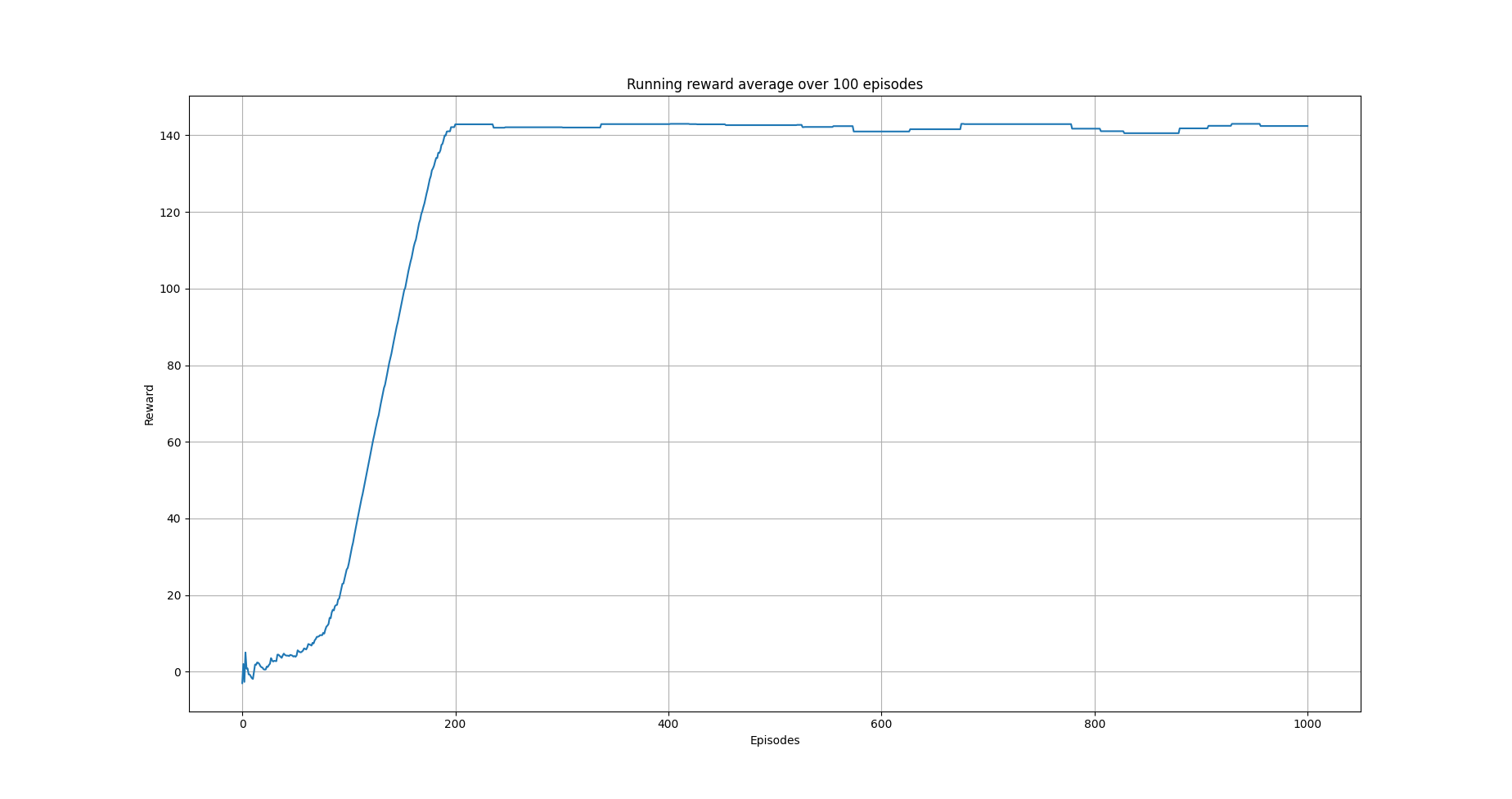
Running average reward.
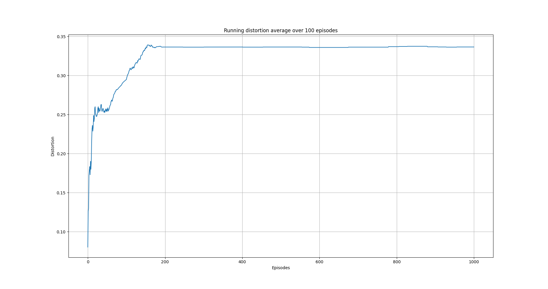
Running average total distortion.
Although there is evidence of learning, it should be noted that this depends heavily on the applied transformations on the columns and the metrics used. So typically, some experimentation should be employed in order to determine the right options.
The following is snapshot of the distorted dataset produced by the agent
ethnicity,salary,diagnosis
British,0.3333333333333333,1
British,0.1111111111111111,0
British,0.5555555555555556,3
British,0.5555555555555556,3
British,0.1111111111111111,0
British,0.1111111111111111,1
British,0.1111111111111111,4
British,0.3333333333333333,3
British,0.1111111111111111,4
British,0.3333333333333333,0
Asian,0.1111111111111111,0
British,0.1111111111111111,0
British,0.1111111111111111,3
White,0.1111111111111111,0
British,0.1111111111111111,3
British,0.3333333333333333,4
Mixed,0.3333333333333333,4
British,0.7777777777777777,1
whilst the following is a snapshot of the distorted dataset by using ARX K-anonymity algorithm
NHSno,given_name,surname,gender,dob,ethnicity,education,salary,mutation_status,preventative_treatment,diagnosis
*,*,*,*,*,White British,*,0.3333333333333333,*,*,1
*,*,*,*,*,White British,*,0.1111111111111111,*,*,0
*,*,*,*,*,White British,*,0.1111111111111111,*,*,1
*,*,*,*,*,White British,*,0.3333333333333333,*,*,3
*,*,*,*,*,White British,*,0.1111111111111111,*,*,4
*,*,*,*,*,White British,*,0.3333333333333333,*,*,0
*,*,*,*,*,Bangladeshi,*,0.1111111111111111,*,*,0
*,*,*,*,*,White British,*,0.1111111111111111,*,*,0
*,*,*,*,*,White other,*,0.1111111111111111,*,*,0
*,*,*,*,*,White British,*,0.3333333333333333,*,*,4
*,*,*,*,*,White British,*,0.7777777777777777,*,*,1
*,*,*,*,*,White British,*,0.1111111111111111,*,*,2
*,*,*,*,*,White British,*,0.1111111111111111,*,*,2
*,*,*,*,*,White other,*,0.1111111111111111,*,*,2
*,*,*,*,*,White British,*,0.5555555555555556,*,*,0
*,*,*,*,*,White British,*,0.5555555555555556,*,*,4
*,*,*,*,*,White British,*,0.5555555555555556,*,*,0
*,*,*,*,*,White British,*,0.3333333333333333,*,*,0
Note that the K-anonymity algorithm removes some rows during the anonymization process, so there is no one-to-one correspondence to the two outpus. Nonetheless, it shows qualitatively what the two algorithms produce.
References
Richard S. Sutton and Andrw G. Barto, Reinforcement Learning. An Introduction 2nd Edition, MIT Press.
Watkins, Learning from delayed rewards, King’s College, Cambridge, Ph.D. thesis, 1989.